This annex documents simple models for first
estimation or screening.
An urban area contains thousands, or even
millions, of individual sources. The application of a diffusion model to each source is
impractical. Consequently most of the small sources are combined into larger area sources
of strength Qa (mass per unit time per unit area), and it is assumed
that the emissions from the ground surface are uniform over that particular area.
Diffusion from the largest point sources can
be calculated individually and the resulting concentrations at a receptor point can be
added to the contribution from the area sources.
A. AREA SOURCE MODEL
In order to estimate by hand calculations the
1hr average air concentration at an arbitrary receptor point (o) due to area source
emissions, a modified expression of the ATDL urban diffusion model (Hanna, 1972; Gifford
and Hanna, 1973) may be used:
 (A.1)
(A.1)
where
C, the concentration (micrograms m-3)
o, denotes the location of the receptor
point
n, is the number of grid blocks (of
size ), necessary to reach the
upwind edge of the urban area, starting from the receptor point.
Q , for i=o,1,2,...,n, are source strengths (microgram sec-1
m-2), constant over a distance
  .
.
u, is the wind speed, assumed constant
within the mixing layer.
c,d are the Brookhaven National
Laboratory parameter values, (Smith, 1968), as listed in Table 1.
Table A.1. Brookhaven National Laboratory parameter values a, b, c
and d in equation (A.1) and in the formulas for the dispersion parameters ,  and
and 
| atmospheric
conditions |
insolation
|
wind speed
|
a
|
b
|
c
|
d
|
| very unstable |
strong-moderate
|
2
|
0.40
|
0.91
|
0.40
|
0.91
|
| unstable |
strong-moderate
|
2-3
|
0.36
|
0.86
|
0.33
|
0.86
|
| neutral |
moderate-slight
|
3-4
|
0.32
|
0.80
|
0.22
|
0.80
|
| estimated Pasquill D |
moderate-slight
or night
|
4
|
0.32
|
0.75
|
0.15
|
0.75
|
| stable |
night
|
2-4
|
0.31
|
0.71
|
0.06
|
0.71
|
Note that these values represent one choice;
alternative datasets exist. Note also the dependence of the dispersion parameters on
averaging time (see end of this annex).
Basic assumptions
- The pollutants are assumed to be uniformly mixed in a
layer, whose height is proportional to the vertical dispersion parameter
 , where x is the total distance
from the urban area.
Simpler approach
When the distribution of emissions is quite
smooth, as it is often the case in residential urban areas, the calculated concentration
(C) at any receptor point is usually proportional to the emissions Qao in the
grid square in which the receptor is located. In this case it is sufficient to use the
following simpler relation:
 (A.2)
(A.2)
the expression  denotes the distance to the edge of
city.
The following values for the dimensionless
factor A are suggested:
| atmospheric conditions |
A
|
| neutral or average |
200 |
| stable |
600 |
| unstable |
50 |
Note, however, that A is slightly dependent
on  .
.
Additional contribution from other sources
The urban area source model can give the
average concentration over a broad area. In a street canyon or adjacent to a highway in an
urban area, there is an additional contribution to the concentration from local sources.
In this case the total concentration Ct is the sum of the spatial
average C (calculated from equation (A.1)) and the local Cl
component. Finally, the concentrations resulting at a receptor point from large point
sources, Cp, can also be added to the spatial average concentration C.
B. ELEVATED POINT SOURCES
In order to estimate the contribution from an
elevated point source Cp, (Fig. 1) of strength Q, the following Gaussian
relation can be used:
 (A.3)
(A.3)
where
C is the concentration (micrograms m-3);
Q is the source strength (micrograms
sec-1);
u is the wind speed at the plume
height;
y refers to the horizontal direction at
right angles to the plume axis with y equal to zero on the axis;
z is the height above the ground;
 are standard deviations of the concentration distribution C, in
the y and z direction and are calculated from table A.1;
h is the effective plume
height (stack height plus plume rise). The plume rise can be calculated by using the
appropriate formulas, summarised in table A.2
. 
Figure A.1 Diagram
of plume, illustrating concepts important in the Gaussian plume formula.
Table A.2. Plume rise
formulas according to the plume characteristics and atmospheric conditions
| plume type |
1 |
atmospheric
conditions
|
formulas
|
|
bent-over
|
buoyant
jet
|
stable
strong wind
neutral,
unstable
strong wind neutral
|


|
| vertical |
jet
buoyant
|
low wind
stable |


|
where
 is the
buoyancy flux ,
  ;
;
M is the momentum flux, M=wV;
s is the atmospheric
stability,  ;
;
V is the plume volume flux (V=wR2
for vertical plume and V=uR2 for bent over plume);
w is the plume vertical speed;
x is distance from the stack;
D is the stack diameter;
T is the temperature.
Subscripts p and e denote plume
and environment.
Note that alternative formulations for the
plume rise exist.
Limitations
Although the Gaussian plume formula in general
is appropriate to calculate the dispersion of elevated continuous major point sources, it
has been demonstrated that it can lead to misleading results in special cases, such as in
inhomogeneous terrain. For other simple models which could be used, see for instance
Kretzschmar et al.,1994; Kretzschmar and Cosemans, 1996.
Longer averaging times
The diffusion parameters  are directly related to the
standard deviations of the turbulent velocity fluctuations. Thus, as averaging time
increases, the turbulent velocity fluctuations increase and hence
  increase. Gifford suggests accounting for the effects of
sampling time trough the empirical formula:
 (A.4)
(A.4)
where,
d and e represent two different averaging
times, and q is in the range 0.25 to 0.3 for 1hrsd<100hr and equals
approximately 0.2 for 3minsd<1hr.
The standard dispersion parameters given in
table A.1, represent a sampling time Tse of about 10 min.
Extension to longer averaging times is made by
solving the above equations for a variety of wind directions and then weighting each
result by the frequency with which the wind blows from that direction.
C. STREET CANYON SUBMODEL
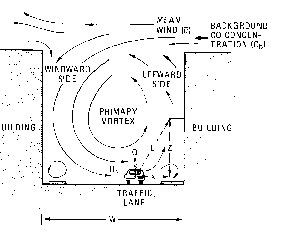
Consider the street canyon in figure
A.2, where the important variables are defined. Depending on the wind direction, at roof
level, the following relations can be used.

Figure A.2 Schematic of
cross-street air circulation in a street canyon. [From Johnson et al, 1977)
Wind direction normal to the street axis
If the wind direction is nearly normal to the
street, the equations for the concentration Cl in the street canyon are:
- lee side,
 (A.5)
(A.5)
- windward side,
 (A.6)
(A.6)
where,
| Cl |
is the concentration (µg/m3); |
| N |
is the traffic flow
(vehicles/hr); |
| q |
is the emission factor (g/km); |
| u |
is the wind speed at roof level
(m/sec); |
| W |
is the street width(m); |
| x and z |
are horizontal distance and
height (both in m) of the receptor point relative to the traffic lane; |
| K |
is a dimensionless "best
fit" constant (K 7 is
suggested). 7 is
suggested). |
Wind direction parallel to the street axis
If the wind direction is nearly parallel to
the street axis, the equations for the concentration Cl in the street
canyon are:
 (A.7)
(A.7)
Limitation: The model as such is not
suitable for calculation of NO2 concentrations, which are mainly determined by
chemical reaction of NO with ozone.
D. HIGHWAY SUBMODEL
The excess concentration Cl contributed
by a major highway in an urban area is important for a distance less than 300m downwind of
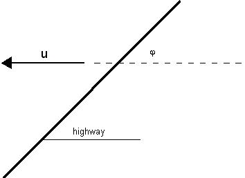
the highway. Consider the highway in figure A.3, the concentration at some distance x
from the highway can be estimated from the relation:
 (A.8)
(A.8)
where
C is the concentration (µg/m3);
Q is the line source strength
(µg/s/m);
h is the effective height of emissions
due to initial dispersion (2-3m);
 is the
angle between the wind direction and the highway;
 is the vertical dispersion parameter.
F( ) Function of
  ; for
; for  around
90 degrees, F(
 ) is close to 1.

Figure A.3 Infinite
line source pattern.
Limitation: This formula cannot be used
to calculate concentrations on the highway, or in case the wind blows in the direction of
the highway .
Meteorological data and emissions
All the models in this annex are best suitable
for estimation of long term average concentrations. They should not be used for short term
high percentile values, which are highly dependent on critical meteorological conditions.
For long term average concentrations,
calculations can be made with average meteorological conditions. For wind speed, the
annual average can be used. For wind direction, the most frequent direction can be taken.
For point sources, neutral atmospheric conditions should be selected.
Appropriate choices must also be made for
emission estimates, to make sure that they reflect typical conditions.
References
Gifford F.A. and Hanna S.R., (1973) Modelling
urban air pollution. Atmospheric Environment, 7, 131-136.
Hanna S.R., (1972) Description of ATDL
computer model for dispersion from multiple sources. Proc. of second annual industrial air
pollution control conference. Knoxville, Tn. ATDL Report 56, NOAA, Oak Ridge.
W. B. Johnson, R. C. Sklarew, and D. B.
Turner, Urban Air Quality Simulation Modeling in Air Pollution, vol. 1, 3rd ed. Chapter
10, p. 530, A. G. Stern (Ed.), Academic Press, New York, 1977.
Kretzschmar, J.G., Cosemans G.(1996) 4th
workshop on harmonization within atmospheric dispersion modelling for regulatory purposes,
vol. 1 and 2. E&M.RA9603, VITO, Mol, Belgium.
Kretzschmar, J.G., Maes, G. Cosemans G.(1994)
Operational short range atmospheric dispersion models for environmental impact assessment
in Europe, vol 1 and 2. E&M.RA9416, VITO, Mol, Belgium.
Smith, M. E. (ed.) (1968) Recommended Guide
for the Prediction of the Dispersion of Airborne Effluents, Am. Soc. of Mech. Engineers,
New York


 (A.3)
(A.3)


 ;
;

 (A.5)
(A.5)
Document Actions
Share with others