This chapter summarises methods for obtaining
a preliminary overview of the air quality situation in a zone by measurements, in the case
that no previous assessment is available. These measurements are not intended to control compliance of limit values under Article 6
of the FWD, but rather are screening techniques meant to determine what compliance
measurements and other assessments are needed to comply to EC legislation. The results of
preliminary measurements can be complemented with an assessment of emission sources and
modelling to obtain a full picture of the air quality in a zone, as measurements are
inherently limited in their representativeness in space and time.
3.2 Measuring strategy
A measuring strategy depends on the
objectives of the monitoring, and the pollutants to be assessed. For the relevant air
quality parameters (concentration of pollutants and associated
averaging time), we need to specify where, how, and how often
measurements should be taken. The measuring effort will be dependent on:
- the variation of pollutant concentrations in
space and time;
- the availability of supplementary information;
- the accuracy of the estimate, that is required.
It is possible to derive, in quantitative
terms, a measuring strategy from this information. However, this is not always
practicable, as the required accuracy is often not specified, and the variation of the
pollutant in space and time may not be sufficiently well known. In this guidance report,
the following approach is proposed:
| 1. |
Estimate the
levels and spatial variation of the quantity from existing measurements in the zone, or in
similar situations elsewhere, or from emission inventories and model calculations. |
| Where measurements are being used as the basis of the assessment, |
| 2. |
Design a
measuring strategy for assessing the spatial distribution of pollutants, the pollutant
levels in areas with highest concentrations and in background locations. |
| 3. |
Carry out
measurements with appropriate methods, with a frequency and over a period of time as
specified below. |
| 4. |
Calculate
from the measurement results estimates of the relevant air quality statistics. |
| 5. |
Estimate the
uncertainty of the measured estimates, taking into account the accuracy of the individual
measurements, station representativeness, and variability of the pollutant in space and
time. |
| 6. |
Where
available compare model estimates and measured estimates, and evaluate discrepancies. |
Steps 2 and 3 are covered in paragraph 3.4,
3.5 and 3.6, steps 4 and 5 in paragraph 3.7. Information on emissions and models is
provided in chapters 4 and 5.
A measuring strategy for preliminary assessment will concentrate on
the question in which areas pollution levels exceed limit values, or the associated
assessment threshold levels, as set by the Directive. For those areas, more intensive
assessment as described in article 6 of the FWD will be required. The preliminary
assessment should not only identify the location of maximum concentrations, but also
determine the extent and the limits of the area of exceedance.
3.3 Preliminary measurement techniques
Currently used air quality measurement techniques
can be sub-divided in three main categories:
manual methods
These are the simplest and cheapest
measurement methods, usually based on a sampling procedure followed by chemical analysis
(or gravimetric determination for suspended particulate matter). According to the
implemented sampling procedure, different manual methods can be recognised: the use of
bubblers for gaseous pollutants, the diffusive sampling method for gaseous pollutants, and
the collection on filters for suspended particulate matter (Black Smoke and PM10) and
heavy metals measurements.
automated methods
These currently constitute the most widespread
monitoring technique in the air quality monitoring networks. The analysis of the
pollutants is based on physical principles and processed electronically. Automated
analysers allow for the continuous, automated, on-line and time-resolved measurement of
air pollutants. The major drawback of this technique resides with the high costs for
purchase and maintenance of the analysers, often resulting, as a consequence, in low
network density and low spatial resolution of the measurements
Mobile laboratories equipped with automated
analysers constitute a useful application of this technique as a tool for measurement
campaigns at locations of interest.
long-path optical methods
such as the Differential Optical Absorption Spectrometry (DOAS), allow for the
simultaneous monitoring of various gaseous pollutants integrated over a distance of
several hundreds of meters. As for the other automated methods, the long-path optical
methods allow for the continuous, automated, on-line and time-resolved measurement of air
pollutants.
Among these measurement techniques, screening
techniques based on the use of a mobile laboratory and the diffusive sampling technique or
other manual methods are of particular interest, because of their relatively low cost and
their simple and fast operation, in comparison with fixed monitoring stations. Three
different approaches are proposed in this chapter:
- the diffusive sampling technique (see 3.4);
- the use of a mobile laboratory in areas of
maximum concentrations (see 3.5);
- the use of a mobile laboratory for grid
measurements (see 3.6).
or a combination of one or more of the
proposed approaches.
3.4 Use of the diffusive
sampling technique
3.4.1 General methodology
The low cost and easy operation of the
diffusive sampling technique make it an ideal tool for large scale air pollution surveys
with a high spatial resolution (De Saeger et al.,1991,1995). A diffusive sampler is a
device capable of taking gas samples from the atmosphere at a rate controlled by molecular
diffusion, and which does not require the active movement of air through the sampler. The
diffusive sampler consists of a tube, one end containing a sorbent which fixes the
pollutant. The pollutant is sampled onto the sorbent at a rate controlled by the molecular
diffusion of the pollutant gas in the air, without requiring any pump or electrical power.
After exposure of the samplers over periods varying from a few days to a few weeks, the
tubes are closed and returned to the laboratory for analysis. According to the type of
device and the measured pollutant, analysis can be performed using different techniques,
such as colorimetry, ion chromatography and others. Maps of the pollutant concentrations
over the area can be obtained by interpolation of the diffusive sampler measurements (see
Fig. 1: Example of Madrid - Spatial distribution of NO2 levels determined by
diffusive sampling) Diffusive samplers are today available for a large number of gaseous
pollutants, such as SO2, NO2, O3, CO, Benzene.
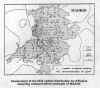
Fig.1 Spatial distribution of NO2 levels determined by diffusive sampling
(example of Madrid)
The technique is particularly suited to
determine the pollutant distribution over a large area, and to assess integrated
concentration levels over longer periods of time (long-term limit values). Short-term
limit values can be derived from statistical data, by comparison with extended and time
resolved measurement series from similar measurement locations. The proposed methodology
can be used to determine areas of maximum concentration and combined with the use of a
mobile laboratory as described in 3.5. In addition it may support the optimisation of
monitoring networks and assessments supporting generalisation.
When applying this methodology in the case of
a preliminary assessment, the following steps are proposed:
- Establish the location of the main emission sources
from an assessment of emission sources.
- Construct a grid over the area under investigation
taking into account the density of the sampling sites specified in the data quality
requirements.
- Select for each cell of the grid a location
representative of the background pollution level in that cell, that is not directly
influenced by local pollution sources.
- If necessary, select additional sampling sites in the
vicinity of important pollution sources (hot spots such as roads with heavy traffic,
industrial sources).
- Install the samplers over the area and expose them
over a representative time period taking into account the minimum time coverage specified
in the data quality requirements included in this guidance.
- In support of the QA/QC of the measurements, it is
recommended to install duplicate/triplicate samplers in a limited number of sites in order
to assess the reproducibility of the measurements. Unexposed samplers should be kept
during the period of exposure for assessing the sampler blank value.
- Perform the analysis of the diffusive samplers in the
laboratory and calculate the pollution levels for each particular site.
- Calculate the distribution of the pollution levels by
interpolation of the measurements made in each grid cell. The measurements performed in
the vicinity of sources (hot spots) are not necessarily representative of a larger area,
and should in that case not be included in the interpolation calculations.
- Make a graphical presentation of the pollutant in map
form. Concentrations measured at hot spots are indicated on the map.
- Estimate percentile values by comparison with
extended and time resolved measurement series from similar measurement locations.
- Compare the obtained measurement results with the
limit values of the directive and select the appropriate assessment regime.
It should be noted that diffusive samplers
are very cost effective, but that their implementation on a large scale may be labour
intensive and hence costly. They can however also be a useful tool when used less
intensively in conjunction with other assessment methods.
Other manual measurement techniques, such as
bubblers (total acidity, Thorin and TCM method for SO2, Saltzmann method for NO2),
can be used as an alternative to the diffusive sampling technique, in particular when the
number of samplers to be implemented is low. The methodology proposed for the diffusive
sampling technique applies in that case also for bubblers.
3.4.2 Data quality requirements
When performing diffusive sampling campaigns,
the following data quality requirements are proposed. These data quality objectives are
only indicative, and may be strengthened where possible.
- Maximum uncertainty of the measurements:
±30% (for single measurements and a 95% confidence interval averaged over the reference
period and at the level of the limit value, taking into account errors of calibration,
sampling efficiency, analytical performances and the effect of environmental parameters).
The measurements should be supported by an adequate QA/QC programme during the period of
the campaigns, and the quality of the measurements should be fully documented.
It should be noted that the diffusive sampling
technique is still coping with a lack of harmonised validation data. The current state of
the art of the technique however has shown that the required uncertainty level (± 30%)
can be met for SO2 and NO2, provided that the measurements be supported by an adequate
QA/QC programme. The European Committee for Standardisation (CEN - Technical Committee 264
- Working Group 11) is currently developing requirements and test methods for the
implementation of the diffusive sampling technique (CEN,1996).
- Siting criteria and number of samplers: The
diffusive samplers should be installed at those sites where the limit values apply
(kerbside, urban background, rural background, etc.). The density of the sampling sites
essentially depends on the spatial variability of the pollution levels, and hence may vary
with type of pollutant, source distribution, local orography and meteorology.
In the case of those agglomerations for which
an intensive measurement campaign is undertaken, it is proposed to install a number of
samplers equal to 15 times the initial number of measurement stations required for
mandatory measurements (Ni). This would result in a number of 30 samplers for
agglomerations with a population of 250.000 inhabitants, of 60 samplers for agglomerations
with a population number of 1.000.000 inhabitants and of 150 samplers for an agglomeration
of 6.000.000 inhabitants (see Daughter Directive proposal for SO2, PM10, NO2
and Pb). The sampler density may vary in function of the emission sources configuration,
and it is good practice to increase the sampler density in city centers with respect to
the outskirts (see Fig. 2: Example of Athens - Construction of the measurement grid).
Additional samplers would be installed at a representative sample of hot spots, such as
along busy roads and crossings, as well as in the surroundings of industrial pollution
sources, in particular if they are likely to affect local pollution levels. A limited
number of samplers should be installed at the periphery of the area under investigation,
in order to assess the impact of adjacent areas.
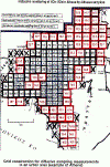
Fig.2 Grid construction for diffusive sampling measurements in an urban area (example of Athens)
In other cases (industrial zones, rural
background), the number of stations should be sufficient to
determine the extent of pollution and exposure.
- Minimum time coverage: 20% of the reference
period of the directive's long-term limit value (1 year), by example five 2 weeks periods
evenly distributed over the year, or two 5 week periods corresponding to the seasons with
maximum and minimum pollution levels (typically during winter and summer periods).
- Minimum data capture: 90% of the time of the
campaigns, allowing for a failure (leakage, theft, vandalism, presence of insects) of the
diffusive samplers during 10% of the time.
3.4.3
Specific information on existing diffusive samplers
Diffusive samplers for ambient air
measurements have been developed for various pollutants. The Palmes diffusion tube for the
measurement of SO2 and NO2 is certainly the best known, but several
other types are widely used today (Palmes, 1973; 1976). Figure 3 gives an example of
currently available diffusive samplers. Other kinds of samplers are today available,
covering almost all the gaseous pollutants foreseen by the Framework Directive
(Brown,1993). A guide for the selection and the application of the diffusive sampling
technique is currently being prepared by CEN - Technical Committee 264 - Working Group 11
(CEN,1996).
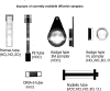
Fig.3 Example of currently available diffusive samplers
The following table gives a
review of the existing diffusive samplers and of their analytical principles:
| Pollutant |
Analytical
principle |
| SO2
|
Chemical absorption
+ colorimetry / ion chromatography |
| NO2 |
idem |
| NOX |
idem (same as for NO2
+ oxidation layer) |
| O3 |
Chemical absorption
+ colorimetry |
| CO |
Chemical absorption
+ colorimetry |
| BENZENE |
Chromatographic
adsorbent + GC analysis |
It should be noted that the principle of
molecular diffusion does not adapt to particulate matter, and that the diffuse sampling
technique is therefore not applicable for PM10 or heavy metals (Plants have been used as
passive samplers for some of these substances, but this is a surrogate for deposition
rather than for concentration measurements).
In urban areas, the spatial variation for
primary pollutants such as NO, CO, Pb, PAH's and benzene is mainly determined by their
emissions from automotive traffic. As a result of this, one single pollutant
representative of the emissions from automotive traffic may be used as indicator for the
other pollutants, when determining areas of maximum concentrations. This
"indicator approach" is however valid only if large industrial sources with low
level emission heights are not present in the area. Particularly for Pb, PAH or benzene,
this cannot be taken for granted. Nor is this approach acceptable for secondary pollutants
such as NO2.
3.5
Use of a mobile laboratory in areas of maximum concentrations
3.5.1 General methodology
The methodology allows evaluation of the
maximum concentration levels in a zone over a period that is representative of the
reference period(s) of the limit value. It is used as a preliminary assessment method in
order to verify whether a zone is in exceedance or near-exceedance of the limit values,
and determine the ongoing assessment regime that will be required under Article 6 of the
Framework Directive.
Mobile laboratories or transportable
measurement stations used for stationary measurements at fixed sites, usually combine the
advantages of automated measurement methods (continuous, time-resolved measurements) with
mobility or flexibility. For pollutants for which automated measurement methods are not
available, mobile laboratories may also be equipped to perform non-automated measurements
(PM10, heavy metals, PAH's). The duration, the periods and the frequency of the campaigns
or measuring periods will have to be established so as to be representative of the
reference period of the limit value (1 hour, 24 hours, 1 year).
The location of maximum concentration levels
in a zone will be chosen taking into account the source distribution, local meteorological
conditions and orography. The types of sources present in an area are very important when
choosing a measuring site. Impact from elevated point sources is often difficult to
measure at one point at ground level because both wind direction and wind speed, and their
variation with height is important for the location of the maximum ground level impact.
For monitoring the pollution from roads, the impact will decrease with the distance from
the road, and the level of pollution will on average be proportional to the volume of
traffic. Time-series of hourly concentrations should reflect the pattern of traffic
intensity. The highest concentrations for 24-hour periods should be expected to be located
in areas where the road runs parallel to the most frequent wind-directions, or where the
curvature of the road allows impact from several wind-directions. For monitoring pollution
mainly from area-sources the location should be chosen close to the centre of the area,
and avoid direct impact from "super local" sources in the vicinity (example:
small incinerators or petrol stations). In complex situations resulting in a high
variability of the pollutant distribution (sources of different origins, complex terrain
and meteorology), it is advisable to perform the measurements in different representative
locations.
When applying this methodology the following
steps are proposed:
- Establish the location of expected maximum
concentration from either existing measurements, from information from similar zones,
emissions inventories or modelling studies. The diffusive sampling technique (see 3.4)
used as a tool to determine the spatial distribution of pollutants, may constitute an
alternative technique to assess the areas of maximum concentration levels.
- From time series of existing measurements or from
information from similar zones, determine the periods of maximum pollution levels.
- Perform the measurements as specified in the data
quality requirements.
- Compare the obtained measurement results with the
limit values of the Directive (see 3.7) and select the appropriate assessment regime.
3.5.2 Data quality requirements
When performing the measurements with a
mobile laboratory, the following data quality requirements are proposed. These data
quality objectives are only indicative, and may be strengthened where possible.
- Maximum uncertainty of the measurements:
±15% for gaseous pollutants and ± 30% for particulate matter measurements (for single
measurements averaged over the reference period and at the level of the limit value,
taking into account errors of sampling, calibration and instrument performances). The
measurements should be supported by an adequate QA/QC programme during the period of the
campaigns (periodic in-situ calibration and calibration check, proper maintenance
of instrumentation), and the quality of the measurements should be
fully documented.
- Minimum time coverage: For long-term limit
values (typically 1 year), 20% of the reference period, by example five 2 weeks periods
evenly distributed over the year, or two 5 week periods corresponding to the seasons with
maximum and minimum pollution levels (typically during winter and summer periods). For
short term limit values (24 hour and shorter), 3 months during the expected period of
increased pollution levels.
- Minimum data capture: 90% of the time of the
campaigns or measurement periods, allowing for a failure of the instrumentation during 10%
of the time.
Better estimates of minimum time coverage can
be calculated from stochastic sampling from an existing series of monitoring data in a
similar situation. This exercise has been carried out in the EC Working Groups on
particulates and on benzene (see position papers, to be published)
3.5.3 Specific information for some pollutants
The mobile laboratory would be equipped
with one analyser for each of the pollutants under consideration. The selected measurement
method shall comply with the reference method of the respective Directives as well as with
the quality objectives. The following table gives an example of possible measurement
methods to be used for the assessment.
| Pollutant |
Measurement
method |
| Sulphur dioxide
|
UV fluorescence |
| Nitrogen dioxide |
Chemiluminescence |
| PM10 |
Sampling on filter +
gravimetry (manual method), beta attenuation, oscillating
micro-balance |
| Lead |
Sampling on filter +
atomic absorption spectrometry, ICP, X-ray fluorescence
(manual method) |
A mobile laboratory can easily combine
measurements of various pollutants, and may constitute a unique screening tool for
pollutants for which cost effective measuring techniques are not available (PM10, heavy
metals).
3.6 Use of a mobile laboratory for grid monitoring
3.6.1 General methodology
Further to the assessment of pollution levels in areas of maximum
concentrations, a mobile laboratory can also be used to assess the pollutant spatial
distribution over a larger area. Grid monitoring is performed by dividing the particular
area of interest into a grid of squares, and by measuring the pollution levels in each
grid cell. The measurements are made during short periods of time at each intersection of
the grid lines, and repeated over the course of a year. The dates and hours for the
measurements are chosen randomly but in such a way that they are evenly distributed over
the months, the days of the weeks and the hours of the day. The measuring schedule is laid
out so that no neighbouring intersections are measured on the same day. The single values
measured at the four corners of each grid are used to calculate the mean concentration
value for each grid cell and the pollutant concentrations isopleths
over the area. Percentile values can be estimated statistically from the
accumulated frequency distribution.
Note that the method is not suitable to characterise air quality hot
spots, for which additional sampling should be carried out.
A typical example of this methodology is illustrated by a study made
in Karlsruhe for NO2, see fig. 4: Example of Karlsruhe - Grid monitoring of NO2
levels (UMEG,1996). In this particular case, the area was divided into a grid with a
density of 1 x 1 km, and half-hourly measurements were repeated 26 times over the year,
resulting in 104 half-hourly measurements for each grid square. The measurements were
performed between 6 a.m. and 10 p.m., resulting in an overestimation of the concentration
levels, but measurements during the night may be considered when a higher accuracy is
necessary.
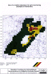
Fig.4 Use of a mobile laboratory for grid monitoring (example of Karlsruhe)
The proposed methodology is of particular interest in cases where a
limited number of measurements are required (small agglomerations), or when other kinds of
screening techniques are not available (SPM).
When applying this methodology in the case of a preliminary assessment, the following steps are proposed:
- Construct a grid over the area under investigation
taking into account the density of the grid specified in the data quality requirements.
- Prepare the measurement schedule, by choosing
randomly over the year, the dates and hours for the measurements in such a way that
they are evenly distributed over the months, the days of the weeks and the hours of the
day, taking care that no neighbouring intersections are measured on the same day.
- Perform the measurements with the mobile laboratory at the
intersection of each grid.
- Calculate the yearly average concentration for each grid cell from
the single values measured at the grid intersections.
- Make a graphical presentation of the pollutant
distribution by means of iso-concentration plots over the area.
- Estimate percentile values by comparison with
extended and time resolved measurement series from similar measurement locations.
- Compare the obtained measurement results with the
limit values of the directive and select the appropriate assessment regime.
3.6.2 Data quality requirements
When performing the measurements, the
following data quality requirements are proposed. These data quality objectives are only
indicative, and may be strengthened where possible:
- Maximum uncertainty of the measurements:
±15% for gaseous pollutants and ± 30% for particulate matter measurements (for single
measurements averaged over the reference period and at the level of the limit value,
taking into account errors of sampling, calibration and instrument performances). The
measurements should be supported by an adequate QA/QC programme during the period of the
campaigns, and the quality of the measurements should be fully documented.
- Minimum time coverage: For long-term limit
values (typically 1 year), 100% of the reference period, randomly spread over all the
measurement sites.
- Minimum data capture: 90% of the time of the
campaigns or measurement periods, allowing for a failure of the instrumentation during 10%
of the time.
- Minimum grid density: In the case of
agglomerations, it is proposed to apply a grid density of 15 times the initial number of
measurement stations required for mandatory measurements (Ni). This would result in a
number of 30 grid cells for agglomerations with a population of 250.000 inhabitants, of 60
grid cells for agglomerations with a population number of 1.000.000 inhabitants and of 150
grid cells for an agglomeration of 6.000.000 inhabitants (see Daughter Directive proposal
for SO2, PM10, NO2 and Pb).
3.6.3 Specific information for 4 first pollutants
See 3.5.3
3.7 Data evaluation and uncertainty assessment
When the measurements have been carried out, the
relevant statistical quantities (annual average, percentile values) for which limit values
are defined, are to be estimated. This is particularly relevant for preliminary
assessments. Particularly for higher percentiles, and for short measuring periods, this
introduces major uncertainties. To our knowledge, no generally accepted methodology is
available; we introduce here some important aspects only.
In principle, the problem may be approached by
assuming a certain frequency distribution of the concentration, and determining the basic
parameters for this distribution. An obvious choice is the log-normal distribution, which
allows for estimation of the median and logarithmic standard deviation, from which all
percentiles can be calculated. Clearly estimates of higher percentiles become
progressively more uncertain in this procedure.
However when estimating these concentration
statistics from the measurements, the following aspects should be considered:
3.7.1 Meteorological variability
The variability of the meteorological parameters
(wind, temperature, atmospheric stability, precipitation, ...) constitute an important
factor affecting the frequency distribution of the measured concentrations. When
calculating the concentration statistics from the measurements, the meteorological
conditions during the measurement period must be checked to be representative of the
normal meteorological conditions, and, if not, the measurements should be corrected
accordingly. The measurements are to be classified according to meteorological classes,
and their weight/frequency adjusted in accordance with the frequency of occurrence of
meteorological classes over a long (10-30 years) period. This method is recommended if the
measurement period is at least one year.
An alternative possibility is:
- Take the same measurement period from a comparable
station with long term continuous measurements
- Compare the statistics for the short term period and
the long term period and calculate correction factors
- Apply these correction factors to the short term,
indicative measurements
3.7.2 Empirical relations for various emission situations
From literature, (semi)-empirical relations may be
found between one hour average concentrations and their longer-term averages (day, month,
year), and relations between those averages and percentiles. However, temporal variations
of concentrations depend a.o. on the source environment, and, consequently, these
relations can be quite different for situations with pollutant emissions from different
source categories (point, line, area). For continuous elevated point-sources, the impact
at one point at ground level will be more dependent upon variability in dispersion
conditions than for line or area sources. The peak-to-mean ratio for a point source is
generally much higher than the ratios for line and area sources. A location where the
pollution level is dominated by contributions from area-sources reflects the variation in
area-source strength with time more than the variations in dispersion conditions.
Estimating concentration statistics from a
limited number of measurements can therefore be a difficult task. The proposed methodology
is best indicated in the case of area- and line-sources, i.e. in urban situations where
the air pollution is diffuse and mainly dominated by automotive and domestic heating
emissions. In the case of point sources, it is generally not possible to assess the
relevant quantities from supplementary measurements. For assessment in these cases, the
combination of emission data and model calculations should be preferred.
3.7.3 Correction for uncertainty of measurements
The impact of measurement uncertainty on
concentration statistics is discussed by Van der Wiel et al. (1988) The variations
related to measuring imprecision introduce upward shifts in the percentiles, which become
increasingly important for higher percentiles. The reliability of this procedure is
dependent on the size of the data base; also, in some cases with rarely occurring high
concentrations, as for example around point sources, the correction may result in even
larger errors.
3.7.4 Uncertainty of individual measurements
The uncertainty of measurements in field conditions
depends on:
- the performances of the measurement system (sampling,
calibration, analysis);
- the expertise of the laboratory responsible for the
measurements or, in practice, the quality system implemented by the laboratory;
- the spatial representativeness of the selected
measurement locations.
Standard testing procedures have been
established to determine the uncertainty of the measurements by a given instrument in
laboratory and field conditions, in particular for type approval of the instrumentation.
It is however far more difficult to estimate the measurement uncertainty in routine field
conditions. This estimation can only be performed experimentally by submitting the
measurement system to quality control in field conditions over a longer period of time
(typically 3 months).
Concerning the spatial representativeness of
the measurement location, a wrong location will undoubtedly lead to an underestimation of
the true concentration, as the measurement strategy is aimed at the measurement of the
highest concentrations. In practice however, it will be impossible to estimate the extent
of the associated uncertainty. It is therefore proposed not to consider this element in
the uncertainty estimation, but to require a detailed report on the siting criteria.
On the basis of experience
obtained from the QA/QC programmes organised by the Joint Research Centre for SO2
and NO2 measurements, an estimation of the uncertainty for measurements made by
a mobile laboratory and by the diffusive sampling technique is given in the following
table (De Saeger, 1996). In both cases, the assumption was made that the laboratory was
implementing a recognised quality system (ISO 9000, EN 45001) and using up to date
instrumentation.
Estimated uncertainty SO2
and NO2 measurements (95% confidence interval)
Source of errors
|
Mobile laboratory (hourly mean value)
|
Diffusive samplers (2-week average)
|
Sampling
Sampling efficiency
Losses in the sampling line |
-5%
|
±15%
|
Calibration chain
Primary calibration
Transfer standard
Calibration check in station |
±10% |
±5% |
Instrument response
Precision, stability, linearity
Selectivity
Environmental variables (T, P, RH %)
Maintenance |
±10 % |
±25 % |
| Propagated uncertainty |
±15% |
±30% |
The regular organisation of quality controls
during the measurement period constitute therefore the only way to contain the uncertainty
of the measurements within the established limits and to document the quality of the
determinations.
3.8 References
- R.H. Brown, "The use of diffusive samplers for monitoring of
ambient air", Pure and Appl. Chem., Vol. 65, N°8, 1859-1874 (1993), © 1993 IUPAC.
- CEN (1996) "Ambient air quality - Diffusive samplers for the
determination of gases or vapours - Requirements and test methods", CEN standard in
preparation, 1996.
- E. De Saeger, M. Gerbolès, M. Payrissat, "La Surveillance du
Dioxyde d'Azote à Madrid au Moyen d'Echantillonneurs Passifs - Evaluation Critique de la
Conception du Réseau", Rapport EUR 4175 FR (1991).
- E. De Saeger, M. Gerbolès, P. Perez Ballesta, L. Amantini, M.
Payrissat, "Air Quality Measurements in Brussels (1993-1994) - NO2 and BTX Monitoring
Campaigns by Diffusive Samplers", EUR Report 16310 EN, 1995.
- E. De Saeger, M. Payrissat, "Quality of air pollution
measurements in the EU monitoring networks". In proceedings of the workshop
"Quality assurance and accreditation of air pollution laboratories", Belgirate,
1996, EUR Report 17698 EN.
- E. D. Palmes, A.F. Gunnisson, "Personal monitoring device for
gaseous contaminants", Am. Ind. Hyg. Assoc. J. 34, 78-81 (1973).
- E. D. Palmes, A.F. Gunnisson, J. Dimattio and C. Tomczyck,
"Personal samplers for nitrogen dioxide", Am. Ind. Hyg. Assoc. J., 37, 570-577
(1976).
- UMEG, Ministerium für Umwelt und Verkehr Baden-Württemberg,
"Umweltschutz in Baden-Württemberg - Luftbericht für den Raum Karlsruhe / Rastatt
1994/95", Bericht UVM-14-96, 1996.
- Van de Wiel, H.J., Eerens, H.C., Van der Meulen, A., (1988), The
impact of measurement uncertainty on air quality characteristics. In: "Air Quality in
Europe", Proceedings of international meeting on harmonization of technical
implementation of EC air Quality Directives, Lyon, 1988. EC, Brussels.

Document Actions
Share with others